Generalized CP (GCP) Tensor Decomposition

Copyright 2022 National Technology & Engineering Solutions of Sandia,
LLC (NTESS). Under the terms of Contract DE-NA0003525 with NTESS, the
U.S. Government retains certain rights in this software.

This document outlines usage and examples for the generalized CP (GCP) tensor decomposition implemented in pyttb.gcp_opt. GCP allows alternate objective functions besides sum of squared errors, which is the standard for CP. The code support both dense and sparse input tensors, but the sparse input tensors require randomized optimization methods.

GCP is described in greater detail in the manuscripts:

D. Hong, T. G. Kolda, J. A. Duersch, Generalized Canonical Polyadic Tensor Decomposition, SIAM Review, 62:133-163, 2020, https://doi.org/10.1137/18M1203626
T. G. Kolda, D. Hong, Stochastic Gradients for Large-Scale Tensor Decomposition. SIAM J. Mathematics of Data Science, 2:1066-1095, 2020, https://doi.org/10.1137/19m1266265

Basic Usage

The idea of GCP is to use alternative objective functions. As such, the most important thing to specify is the objective function.

The command

M = ttb.gcp_opt(data=X, rank=rank, objective=Objectives.<TYPE>, optimizer=<OPT>)

computes an estimate of the best rank-\(R\) generalized CP (GCP) decomposition of the tensor X for the specified generalized loss function specified by <TYPE> solved with optimizer <OPT>. The input X can be a dense tensor or a sparse sptensor. The result M is a Kruskal tensor (ktensor).

Predefined objective functions are:

GAUSSIAN: Gaussian distribution (see also cp_als and cp_opt)
BERNOULLI_ODDS: Bernoulli distribution for binary data
BERNOULLI_LOGIT: Bernoulli distribution for binary data with log link
POISSON: Poisson distribution for count data (see also cp_apr)
POISSON_LOG: Poisson distribution for count data with log link
RAYLEIGH: Rayleigh distribution for nonnegative continuous data
GAMMA: Gamma distribution for nonnegative continuous data
HUBER: Similar to Gaussian but robust to outliers
NEGATIVE_BINOMIAL: Models the number of trials required before we experience some number of failures. May be a useful alternative when Poisson is overdispersed.
BETA: Generalizes exponential family of loss functions.

Alternatively, a user can supply one’s own objective function as a tuple of function_handle, gradient_handle, and lower_bound.

Supported optimizers are:

LBFGSB: bound-constrained limited-memory BFGS (L-BFGS-B). L-BFGS-B can only be used for dense tensors.
SGD: Stochastic gradient descent (SGD). Can be used with both dense tensors and sparse sptensors.
Adagrad: Adaptive gradients SGD method. Can be used with both dense tensors and sparse sptensors.
Adam: Momentum-based SGD method. Can be used with both dense tensors and sparse sptensors.

Each methods has parameters, which are described below.

Specifying Missing or Incomplete Data Using the Mask Option

If some entries of the tensor are unknown, the method can mask off that data during the fitting process. To do so, specify a mask tensor W that is the same shape as the data tensor X. The mask tensor should be 1 if the entry in X is known and 0 otherwise. The call is

M = ttb.gcp_opt(data=X, rank=rank, objective=Objectives.<TYPE>, optimizer=LBFGSB, mask=W)

Note: that mask isn’t supported for stochastic solves.

Solver options

Defaults are listed in brackets {}

Common options that can be passed to pyttb.gcp_opt() include:

init: Initial solution to the problem {“random”}.
printitn: Controls verbosity of printing throughout the solve: print every n iterations; 0 for no printing.
sampler: Class that defined sampling strategy for stochastic solves.

Other Options

In addition to the options above, the behavior of optimizers can be affected by constructing the optimizer with the following optional parameters.

Specifying L-BFGS-B Parameters

m: {None}
factr: Tolerance on the change on the objective value. Defaults to 1e7, which is multiplied by machine epsilon. {1e7}
pgtol: Projected gradient tolerance, defaults to 1e-4 times total tensor shape. It can sometimes be useful to increase or decrease pgtol depending on the objective function and shape of the tensor. {None}
epsilon: {None}
iprint: {None}
disp: {None}
maxfun: {None}
maxiter: {1000}
callback: {None}
maxls: {None}

Specifying SGD, Adagrad, and ADAM Parameters

There are a number of parameters that can be adjusted for SGD and ADAM.

Stochastic Gradient

There are three different sampling methods for computing the stochastic gradient:

Uniform - Entries are selected uniformly at random. Default for dense tensors.
Stratified - Zeros and nonzeros are sampled separately, which is recommended for sparse tensors. Default for sparse tensors.
Semi-Stratified - Modification to stratified sampling that avoids rejection sampling for better efficiency at the cost of potentially higher variance.

The options corresponding to these are as follows.

gradient_sampler: Type of sampling to use for stochastic gradient. Specified by setting pyttb.gcp.samplers.<SAMPLER>. Predefined options for <SAMPLER> are:
- Samplers.UNIFORM: default for dense.
- Samplers.STRATIFIED: default for sparse.
- Samplers.SEMISTRATIFIED
gradient_samples: The number of samples for stochastic gradient can be specified as either an int or a StratifiedCount object. This should generally be \(O(R\sum_{k=1}^d n_k)\), where \(n_k\) is the number of rows in the \(k\)-th mode and \(R\) is the target rank. For the uniform sampler, only an int can be provided. For the stratified or semi-stratified sampler, this can be two numbers a, b provided as arguments to a pyttb.gcp.samplers.StratifiedCount(a, b) object. The first a is the number of nonzero samples and the second b is the number of zero samples. If only one number is specified, then this is used as the number for both nonzeros and zeros, and the total number of samples is 2x what is specified.

Estimating the Function.

We also use sampling to estimate the function value.

function_sampler: This can be any of the three samplers specified above or a custom function handle. The custom function handle is primarily useful in reusing the same sampled elements across different tests.
function_samples: Number of samples to estimate function. As before, the number of samples for estimating the function can be specified as either an int or a StratifiedCount object. This should generally be somewhat large since we want this sample to generate a reliable estimate of the true function value.

Creating the sampler takes two additional options:

max_iters: Maximum number of iterations to normalize number of samples. {1000}
over_sample_rate: Ratio of extra samples to take to account for bad draws. {1.1}

There are some other options that are needed for SGD: the learning rate and a decrease schedule. Our schedule is very simple - we decrease the rate if there is no improvement in the approximate function value after an epoch. After a specified number of decreases (max_fails), we quit.

rate: Rate of descent, proportional to step size. {1e-3}
decay: How much to decrease step size on failed epochs. {0.1}
max_fails: How many failed epochs before terminating the solve. {1}
epoch_iters: Number of steps to take per epoch. {1000}
f_est_tol: Tolerance for function estimate changes to terminate solve. {-inf}
max_iters: Maximum number of epochs. {1000}
printitn: Controls verbosity of information during solve. {1}

There are some options that are specific to ADAM and generally needn’t change:

beta_1: Adam-specific momentum parameter beta_1. {0.9}
beta_2: Adam-specific momentum parameter beta_2. {0.999}
epsilon: Adam-specific momentum parameter to avoid division by zero. {1e-8}

import os
import sys
import pyttb as ttb
import numpy as np

from pyttb.gcp.fg_setup import function_type, setup
from pyttb.gcp.handles import Objectives
from pyttb.gcp.optimizers import LBFGSB, SGD, Adagrad, Adam
from pyttb.gcp.samplers import GCPSampler

Example with Gaussian distribution

X = ttb.tenones((2, 2))
X[0, 1] = 0.0
X[1, 0] = 0.0
rank = 2

Run GCP-OPT

%%time
# Select Gaussian objective
objective = Objectives.GAUSSIAN

# Select LBFGSB solver with 2 max iterations
optimizer = LBFGSB(maxiter=2, iprint=1)

# Compute rank-2 GCP approximation to X with GCP-OPT
# Return result, initial guess, and runtime information
np.random.seed(0)  # Creates consistent initial guess
result_lbfgs, initial_guess, info_lbfgs = ttb.gcp_opt(
    data=X, rank=rank, objective=objective, optimizer=optimizer
)

print(
    f"\nFinal fit: {1 - np.linalg.norm((X-result_lbfgs.full()).double())/X.norm()} (for comparison to f(x) in CP-ALS)\n"
)

WARNING:root:Selected no copy, but input factor matrices aren't F ordered so must copy.

WARNING:root:Selected no copy, but input factor matrices aren't F ordered so must copy.

 This problem is unconstrained.
WARNING:root:Selected no copy, but input factor matrices aren't F ordered so must copy.

WARNING:root:Selected no copy, but input factor matrices aren't F ordered so must copy.

RUNNING THE L-BFGS-B CODE

           * * *

Machine precision = 2.220D-16
 N =            8     M =           10

At X0         0 variables are exactly at the bounds

At iterate    0    f=  1.23602D+00    |proj g|=  9.67634D-01

At iterate    1    f=  1.00610D+00    |proj g|=  9.82961D-02

At iterate    2    f=  1.00136D+00    |proj g|=  7.09402D-02

           * * *

Tit   = total number of iterations
Tnf   = total number of function evaluations
Tnint = total number of segments explored during Cauchy searches
Skip  = number of BFGS updates skipped
Nact  = number of active bounds at final generalized Cauchy point
Projg = norm of the final projected gradient
F     = final function value

           * * *

   N    Tit     Tnf  Tnint  Skip  Nact     Projg        F
    8      2      4      1     0     0   7.094D-02   1.001D+00
  F =   1.0013595802774788     

STOP: TOTAL NO. of ITERATIONS REACHED LIMIT                 

Final fit: 0.2924126978677901 (for comparison to f(x) in CP-ALS)

CPU times: user 8.17 ms, sys: 19 µs, total: 8.19 ms
Wall time: 8.37 ms

Compare to CP-ALS, which should usually be faster

%%time
result_als, _, info_als = ttb.cp_als(
    input_tensor=X, rank=rank, maxiters=2, init=initial_guess
)
print(
    f"\nFinal fit: {1 - np.linalg.norm((X-result_als.full()).double())/X.norm()} (for comparison to f(x) in GCP-OPT)\n"
)

CP_ALS:
 Iter 0: f = 9.999999e-01 f-delta = 1.0e+00
 Iter 1: f = 9.999999e-01 f-delta = 4.5e-08
 Final f = 9.999999e-01

Final fit: 0.9999999999999946 (for comparison to f(x) in GCP-OPT)

CPU times: user 2.07 ms, sys: 190 µs, total: 2.26 ms
Wall time: 2.14 ms

Now let’s try is with the ADAM functionality

%%time
# Select Gaussian objective
objective = Objectives.GAUSSIAN

# Select Adam solver with 2 max iterations
optimizer = Adam(max_iters=2)

# Compute rank-2 GCP approximation to X with GCP-OPT
# Return result, initial guess, and runtime information
result_adam, _, info_adam = ttb.gcp_opt(
    data=X,
    rank=rank,
    objective=objective,
    optimizer=optimizer,
    init=initial_guess,
    printitn=1,
)
print(
    f"\nFinal fit: {1 - np.linalg.norm((X-result_adam.full()).double())/X.norm()} (for comparison to f(x) in GCP-OPT & CP-ALS)\n"
)

Final fit: 0.9999964005920317 (for comparison to f(x) in GCP-OPT & CP-ALS)

CPU times: user 609 ms, sys: 12.4 ms, total: 621 ms
Wall time: 605 ms

# Inspect runtime information from each run
print(f"Runtime information from `gcp_opt_lbfgs`: \n{info_lbfgs}")
print(f"\nRuntime information from `cp_als`: \n{info_als}")
print(f"\nRuntime information from `gcp_opt_adam`: \n{info_adam}")

Runtime information from `gcp_opt_lbfgs`: 
{'grad': array([-0.02339697,  0.00449126, -0.00423005, -0.02089828,  0.05503584,
       -0.07094022, -0.05661871,  0.02955359]), 'task': 'STOP: TOTAL NO. of ITERATIONS REACHED LIMIT', 'funcalls': 4, 'nit': 2, 'warnflag': 1, 'final_f': 1.0013595802774788, 'callback': {'time_trace': array([0.00520651, 0.00673018])}, 'main_time': 0.0069800090004719095}

Runtime information from `cp_als`: 
{'params': {'stoptol': 0.0001, 'maxiters': 2, 'dimorder': array([0, 1]), 'optdims': array([0, 1]), 'printitn': 1, 'fixsigns': True}, 'iters': 1, 'normresidual': np.float64(7.884953353001448e-08), 'fit': np.float64(0.9999999442449602)}

Runtime information from `gcp_opt_adam`: 
{'f_est_trace': array([0.60997726, 0.02477642]), 'step_trace': array([0.   , 0.001]), 'time_trace': array([1.72919001e-04, 3.05183298e-01]), 'n_epoch': 1, 'main_time': 0.6045142820003093}

Create an example Rayleigh tensor model and data instance.

Consider a tensor that is Rayleigh-distributed. This means its entries are all nonnegative. First, we generate such a tensor with low-rank structure.

rng = np.random.default_rng(65)
rank = 3
shape = (50, 60, 70)
ndims = len(shape)

# Create factor matrices that correspond to smooth sinusidal factors
U = []
for k in np.arange(ndims):
    V = 1.1 + np.cos(
        (2 * np.pi / shape[k] * np.arange(shape[k])[:, np.newaxis])
        * np.arange(1, rank + 1)
    )
    U.append(V[:, rng.permutation(rank)])

M_true = ttb.ktensor(U).normalize()


def make_rayleigh(X):
    xvec = X.reshape((np.prod(X.shape), 1))
    rayl = rng.rayleigh(size=xvec.shape)
    yvec = rayl * xvec.data
    Y = ttb.tensor(yvec, shape=X.shape)
    return Y


X = make_rayleigh(M_true.full())

Run GCP-OPT

%%time
# Select Rayleigh objective
objective = Objectives.RAYLEIGH

# Select LBFGSB solver
optimizer = LBFGSB(maxiter=2, iprint=1)

# Compute rank-3 GCP approximation to X with GCP-OPT
result_lbfgs, initial_guess, info_lbfgs = ttb.gcp_opt(
    data=X, rank=rank, objective=objective, optimizer=optimizer, printitn=1
)

print(f"\nFinal fit: {1 - np.linalg.norm((X-result_lbfgs.full()).double())/X.norm()}\n")

WARNING:root:Selected no copy, but input factor matrices aren't F ordered so must copy.

WARNING:root:Selected no copy, but input factor matrices aren't F ordered so must copy.

WARNING:root:Selected no copy, but input factor matrices aren't F ordered so must copy.

RUNNING THE L-BFGS-B CODE

           * * *

Machine precision = 2.220D-16
 N =          540     M =           10

At X0         0 variables are exactly at the bounds

At iterate    0    f=  3.45174D+06    |proj g|=  2.07694D+07

At iterate    1    f=  1.89718D+06    |proj g|=  3.47303D+05

At iterate    2    f=  1.83720D+06    |proj g|=  3.03296D+05

           * * *

Tit   = total number of iterations
Tnf   = total number of function evaluations
Tnint = total number of segments explored during Cauchy searches
Skip  = number of BFGS updates skipped
Nact  = number of active bounds at final generalized Cauchy point
Projg = norm of the final projected gradient
F     = final function value

           * * *

   N    Tit     Tnf  Tnint  Skip  Nact     Projg        F
  540      2      3     32     0     0   3.033D+05   1.837D+06
  F =   1837200.8340656874     

STOP: TOTAL NO. of ITERATIONS REACHED LIMIT                 

Final fit: 0.08931057293468403

CPU times: user 47.5 ms, sys: 8 ms, total: 55.5 ms
Wall time: 31.3 ms

Now let’s try is with the scarce functionality - this leaves out all but 10% of the data!

# Select Rayleigh objective
objective = Objectives.RAYLEIGH

# Select Adam solver
optimizer = Adam(max_iters=2)

# Compute rank-3 GCP approximation to X with GCP-OPT
result_adam, initial_guess, info_adam = ttb.gcp_opt(
    data=X, rank=rank, objective=objective, optimizer=optimizer, printitn=1
)

print(f"\nFinal fit: {1 - np.linalg.norm((X-result_adam.full()).double())/X.norm()}\n")

Final fit: 0.42653557149577837

Boolean tensor.

The model will predict the odds of observing a 1. Recall that the odds related to the probability as follows. If \(p\) is the probability and \(r\) is the odds, then \(r = p / (1-p)\). Higher odds indicates a higher probability of observing a one.

rng = np.random.default_rng(7639)
rank = 3
shape = (60, 70, 80)
ndims = len(shape)

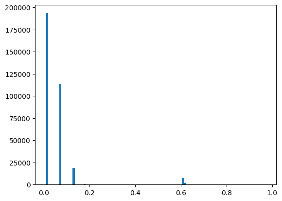
We assume that the underlying model tensor has factor matrices with only a few “large” entries in each column. The small entries should correspond to a low but nonzero entry of observing a 1, while the largest entries, if multiplied together, should correspond to a very high likelihood of observing a 1.

probrange = np.array([0.01, 0.99])
oddsrange = probrange / (1 - probrange)
smallval = np.power(np.min(oddsrange) / rank, (1 / ndims))
largeval = np.power(np.max(oddsrange) / rank, (1 / ndims))

A = []
for k in np.arange(ndims):
    A.append(smallval * np.ones((shape[k], rank)))
    nbig = 5
    for j in np.arange(rank):
        p = rng.permutation(shape[k])
        A[k][p[: nbig - 1], j] = largeval

M_true = ttb.ktensor(A)

Convert `ktensor` to an observed `tensor`. Get the model values, which correspond to odds of observing a 1

Mfull = M_true.double()
# Convert odds to probabilities
Mprobs = Mfull / (1 + Mfull)
# Flip a coin for each entry, with the probability of observing a one
# dictated by Mprobs
Xfull = 1.0 * (ttb.tenrand(shape) < Mprobs)
# Convert to sparse tensor, real-valued 0/1 tensor since it was constructed
# to be sparse
X = Xfull.to_sptensor()
print(f"Proportion of nonzeros in X is {100*X.nnz / np.prod(shape):.2f}%\n");

Proportion of nonzeros in X is 5.55%

Just for fun, let’s visualize the distribution of the probabilities in the model `tensor`.

import matplotlib.pyplot as plt

h = plt.hist(Mprobs.flatten(), bins=100)

../_images/a1d8dd658d029ad441def9e8e1b8520292f24ceb16ef50ec4e7ad2dbedc31b45.png

Call GCP-OPT on the full `tensor`

%%time
# Select Gaussian objective
objective = Objectives.BERNOULLI_ODDS

# Select LBFGSB solver
optimizer = LBFGSB(iprint=1, maxiter=2)

# Compute rank-3 GCP approximation to X with GCP-OPT
result_lbfgs, initial_guess, info_lbfgs = ttb.gcp_opt(
    data=Xfull, rank=rank, objective=objective, optimizer=optimizer
)

print(f"\nFinal fit: {1 - np.linalg.norm((X-result_lbfgs.full()).double())/X.norm()}\n")

WARNING:root:Selected no copy, but input factor matrices aren't F ordered so must copy.

WARNING:root:Selected no copy, but input factor matrices aren't F ordered so must copy.

WARNING:root:Selected no copy, but input factor matrices aren't F ordered so must copy.

WARNING:root:Selected no copy, but input factor matrices aren't F ordered so must copy.

WARNING:root:Selected no copy, but input factor matrices aren't F ordered so must copy.

RUNNING THE L-BFGS-B CODE

           * * *

Machine precision = 2.220D-16
 N =          630     M =           10

At X0         0 variables are exactly at the bounds

At iterate    0    f=  9.27280D+04    |proj g|=  3.36746D+03

At iterate    1    f=  9.18743D+04    |proj g|=  3.08139D+02

At iterate    2    f=  8.54669D+04    |proj g|=  3.36834D+02

           * * *

Tit   = total number of iterations
Tnf   = total number of function evaluations
Tnint = total number of segments explored during Cauchy searches
Skip  = number of BFGS updates skipped
Nact  = number of active bounds at final generalized Cauchy point
Projg = norm of the final projected gradient
F     = final function value

           * * *

   N    Tit     Tnf  Tnint  Skip  Nact     Projg        F
  630      2      5    587     0    23   3.368D+02   8.547D+04
  F =   85466.880845881722     

STOP: TOTAL NO. of ITERATIONS REACHED LIMIT                 

Final fit: -0.17585132842294593

CPU times: user 112 ms, sys: 27.8 ms, total: 140 ms
Wall time: 75.4 ms

Call GCP-OPT on a `sptensor`

%%time
# Select Gaussian objective
objective = Objectives.BERNOULLI_ODDS

# Select Adam solver
optimizer = Adam(max_iters=2)

# Compute rank-3 GCP approximation to X with GCP-OPT
result_adam, initial_guess, info_adam = ttb.gcp_opt(
    data=X, rank=rank, objective=objective, optimizer=optimizer, printitn=1
)

print(f"\nFinal fit: {1 - np.linalg.norm((X-result_adam.full()).double())/X.norm()}\n")

Final fit: -0.045721944151986715

CPU times: user 2.38 s, sys: 0 ns, total: 2.38 s
Wall time: 2.28 s

Create and test a Poisson count `tensor`.

We follow the general procedure outlined by E. C. Chi and T. G. Kolda, On Tensors, Sparsity, and Nonnegative Factorizations, arXiv:1112.2414 [math.NA], December 2011 (http://arxiv.org/abs/1112.2414).

# Pick the shape and rank
sz = (10, 8, 6)
R = 5

# Generate factor matrices with a few large entries in each column
# this will be the basis of our solution.
np.random.seed(0)  # Set seed for reproducibility
A = []
for n in range(len(sz)):
    A.append(np.random.uniform(size=(sz[n], R)))
    for r in range(R):
        p = np.random.permutation(sz[n])
        nbig = round((1 / R) * sz[n])
        A[-1][p[0:nbig], r] *= 100
weights = np.random.uniform(size=(R,))
S = ttb.ktensor(A, weights)
S.normalize(sort=True, normtype=1)

X = S.to_tensor()
X.data = np.floor(np.abs(X.data))

Loss function for Poisson negative log likelihood with identity link.

%%time
# Select Gaussian objective
objective = Objectives.POISSON

# Select Adam solver
optimizer = Adam(max_iters=2)

# Compute rank-3 GCP approximation to X with GCP-OPT
result_adam, initial_guess, info_adam = ttb.gcp_opt(
    data=X, rank=rank, objective=objective, optimizer=optimizer, printitn=1
)

print(f"\nFinal fit: {1 - np.linalg.norm((X-result_adam.full()).double())/X.norm()}\n")

Final fit: -0.10486790906929278

CPU times: user 1.01 s, sys: 0 ns, total: 1.01 s
Wall time: 935 ms

Generalized CP (GCP) Tensor Decomposition

Basic Usage

Specifying Missing or Incomplete Data Using the Mask Option

Solver options

Other Options

Specifying L-BFGS-B Parameters

Specifying SGD, Adagrad, and ADAM Parameters

Stochastic Gradient

Estimating the Function.

Example with Gaussian distribution

Run GCP-OPT

Compare to CP-ALS, which should usually be faster

Now let’s try is with the ADAM functionality

Create an example Rayleigh tensor model and data instance.

Run GCP-OPT

Now let’s try is with the scarce functionality - this leaves out all but 10% of the data!

Boolean tensor.

Convert ktensor to an observed tensor. Get the model values, which correspond to odds of observing a 1

Just for fun, let’s visualize the distribution of the probabilities in the model tensor.

Call GCP-OPT on the full tensor

Call GCP-OPT on a sptensor

Create and test a Poisson count tensor.

Loss function for Poisson negative log likelihood with identity link.

Convert `ktensor` to an observed `tensor`. Get the model values, which correspond to odds of observing a 1

Just for fun, let’s visualize the distribution of the probabilities in the model `tensor`.

Call GCP-OPT on the full `tensor`

Call GCP-OPT on a `sptensor`

Create and test a Poisson count `tensor`.