Tucker Tensors
Copyright 2022 National Technology & Engineering Solutions of Sandia,
LLC (NTESS). Under the terms of Contract DE-NA0003525 with NTESS, the
U.S. Government retains certain rights in this software.
Tucker format is a decomposition of a tensor \(\mathcal{X}\) as the product of a core tensor \(\mathcal{G}\) and matrices (e.g., \(A\), \(B\), \(C\)) in each dimension. In other words, a tensor \(\mathcal{X}\) is expressed as:
\( \mathcal{X} = \mathcal{G} \times_1 A \times_2 B \times_3 C \)
In MATLAB notation: X=ttm(G,{A,B,C})
import pyttb as ttb
import numpy as np
# Upcoming ttensors will be generated with this same initialization.
def generate_sample_ttensor() -> ttb.ttensor:
    np.random.seed(0)
    core = ttb.tensor(np.random.rand(3, 2, 1), shape=(3, 2, 1))  # The core tensor.
    U = [
        np.random.rand(5, 3),
        np.random.rand(4, 2),
        np.random.rand(3, 1),
    ]  # The factor matrices.
    X = ttb.ttensor(core, U)  # Create the ttensor.

    return X


X = generate_sample_ttensor()  # Create the ttensor.
X
Tensor of shape: (5, 4, 3)
	Core is a
		tensor of shape (3, 2, 1) with order F
		data[:, :, 0] =
		[[0.5488135  0.71518937]
		 [0.60276338 0.54488318]
		 [0.4236548  0.64589411]]
	U[0] =
		[[0.43758721 0.891773   0.96366276]
		 [0.38344152 0.79172504 0.52889492]
		 [0.56804456 0.92559664 0.07103606]
		 [0.0871293  0.0202184  0.83261985]
		 [0.77815675 0.87001215 0.97861834]]
	U[1] =
		[[0.79915856 0.46147936]
		 [0.78052918 0.11827443]
		 [0.63992102 0.14335329]
		 [0.94466892 0.52184832]]
	U[2] =
		[[0.41466194]
		 [0.26455561]
		 [0.77423369]]
Creating a ttensor with a tensor core
Alternate core formats: sptensor or tensor
np.random.seed(0)
sptensor_core = ttb.sptenrand([3, 2, 1], nonzeros=3)  # Create a 3 x 2 x 1 sptensor.
U = [
    np.random.rand(5, 3),
    np.random.rand(4, 2),
    np.random.rand(3, 1),
]  # The factor matrices.
Y = ttb.ttensor(sptensor_core, U)  # Core is a sptensor.
Y
Tensor of shape: (5, 4, 3)
	Core is a
		sparse tensor of shape (3, 2, 1) with 3 nonzeros and order F
		[0, 1, 0] = 0.9446689170495839
		[2, 0, 0] = 0.5218483217500717
		[2, 1, 0] = 0.4146619399905236
	U[0] =
		[[0.26455561 0.77423369 0.45615033]
		 [0.56843395 0.0187898  0.6176355 ]
		 [0.61209572 0.616934   0.94374808]
		 [0.6818203  0.3595079  0.43703195]
		 [0.6976312  0.06022547 0.66676672]]
	U[1] =
		[[0.67063787 0.21038256]
		 [0.1289263  0.31542835]
		 [0.36371077 0.57019677]
		 [0.43860151 0.98837384]]
	U[2] =
		[[0.10204481]
		 [0.20887676]
		 [0.16130952]]
dense_tensor = ttb.tensor(np.random.rand(3, 2, 1), (3, 2, 1))  # Core is a tensor.
U = [
    np.random.rand(5, 3),
    np.random.rand(4, 2),
    np.random.rand(3, 1),
]  # The factor matrices.
Y = ttb.ttensor(dense_tensor, U)  # Create the ttensor.
Y
Tensor of shape: (5, 4, 3)
	Core is a
		tensor of shape (3, 2, 1) with order F
		data[:, :, 0] =
		[[0.65310833 0.2532916 ]
		 [0.46631077 0.24442559]
		 [0.15896958 0.11037514]]
	U[0] =
		[[0.65632959 0.13818295 0.19658236]
		 [0.36872517 0.82099323 0.09710128]
		 [0.83794491 0.09609841 0.97645947]
		 [0.4686512  0.97676109 0.60484552]
		 [0.73926358 0.03918779 0.28280696]]
	U[1] =
		[[0.12019656 0.2961402 ]
		 [0.11872772 0.31798318]
		 [0.41426299 0.0641475 ]
		 [0.69247212 0.56660145]]
	U[2] =
		[[0.26538949]
		 [0.52324805]
		 [0.09394051]]
Creating a one-dimensional ttensor
np.random.seed(0)
dense_tensor = ttb.tensor(2 * np.random.rand(2, 1), (2,))  # Core tensor.
Z = ttb.ttensor(dense_tensor, [np.random.rand(4, 2)])  # One-dimensional ttensor.
Z
Tensor of shape: (4,)
	Core is a
		tensor of shape (2,) with order F
		data[:] =
		[1.09762701 1.43037873]
	U[0] =
		[[0.60276338 0.54488318]
		 [0.4236548  0.64589411]
		 [0.43758721 0.891773  ]
		 [0.96366276 0.38344152]]
Constituent parts of a ttensor
X = generate_sample_ttensor()  # Create the ttensor.
X.core  # Core tensor.
tensor of shape (3, 2, 1) with order F
data[:, :, 0] =
[[0.5488135  0.71518937]
 [0.60276338 0.54488318]
 [0.4236548  0.64589411]]
X.factor_matrices # List of matrices.
[array([[0.43758721, 0.891773  , 0.96366276],
        [0.38344152, 0.79172504, 0.52889492],
        [0.56804456, 0.92559664, 0.07103606],
        [0.0871293 , 0.0202184 , 0.83261985],
        [0.77815675, 0.87001215, 0.97861834]]),
 array([[0.79915856, 0.46147936],
        [0.78052918, 0.11827443],
        [0.63992102, 0.14335329],
        [0.94466892, 0.52184832]]),
 array([[0.41466194],
        [0.26455561],
        [0.77423369]])]
Creating a ttensor from its constituent parts
X = generate_sample_ttensor()  # Create the ttensor.
Y = ttb.ttensor(X.core, X.factor_matrices)  # Recreate a ttensor from its parts.
Y
Tensor of shape: (5, 4, 3)
	Core is a
		tensor of shape (3, 2, 1) with order F
		data[:, :, 0] =
		[[0.5488135  0.71518937]
		 [0.60276338 0.54488318]
		 [0.4236548  0.64589411]]
	U[0] =
		[[0.43758721 0.891773   0.96366276]
		 [0.38344152 0.79172504 0.52889492]
		 [0.56804456 0.92559664 0.07103606]
		 [0.0871293  0.0202184  0.83261985]
		 [0.77815675 0.87001215 0.97861834]]
	U[1] =
		[[0.79915856 0.46147936]
		 [0.78052918 0.11827443]
		 [0.63992102 0.14335329]
		 [0.94466892 0.52184832]]
	U[2] =
		[[0.41466194]
		 [0.26455561]
		 [0.77423369]]
Creating an empty ttensor
X = ttb.ttensor()  # Empty ttensor.
X
Tensor of shape: ()
	Core is a
		empty tensor of shape ()
		data = []
Use full or to_tensor to convert a ttensor to a tensor
X = generate_sample_ttensor()  # Create a ttensor.
X
Tensor of shape: (5, 4, 3)
	Core is a
		tensor of shape (3, 2, 1) with order F
		data[:, :, 0] =
		[[0.5488135  0.71518937]
		 [0.60276338 0.54488318]
		 [0.4236548  0.64589411]]
	U[0] =
		[[0.43758721 0.891773   0.96366276]
		 [0.38344152 0.79172504 0.52889492]
		 [0.56804456 0.92559664 0.07103606]
		 [0.0871293  0.0202184  0.83261985]
		 [0.77815675 0.87001215 0.97861834]]
	U[1] =
		[[0.79915856 0.46147936]
		 [0.78052918 0.11827443]
		 [0.63992102 0.14335329]
		 [0.94466892 0.52184832]]
	U[2] =
		[[0.41466194]
		 [0.26455561]
		 [0.77423369]]
X.full() # Converts to a tensor.
tensor of shape (5, 4, 3) with order F
data[:, :, 0] =
[[0.66497416 0.45354281 0.39917702 0.77210991]
 [0.50252742 0.34644731 0.30417958 0.58375429]
 [0.48119404 0.3381225  0.29560878 0.55942684]
 [0.25371838 0.16355973 0.14584965 0.29392047]
 [0.77085415 0.52368038 0.46132233 0.89490068]]
data[:, :, 1] =
[[0.42425559 0.28936173 0.25467618 0.49260853]
 [0.32061407 0.22103447 0.19406752 0.37243706]
 [0.3070033  0.21572321 0.18859932 0.35691607]
 [0.16187312 0.10435162 0.09305254 0.18752218]
 [0.49180735 0.33410972 0.29432509 0.57094943]]
data[:, :, 2] =
[[1.24160273 0.84682989 0.74532111 1.44164064]
 [0.93829123 0.64686714 0.56794717 1.08995351]
 [0.89845873 0.63132351 0.55194425 1.04453065]
 [0.47372884 0.30538962 0.27232236 0.54879195]
 [1.43929596 0.97778686 0.86135538 1.67090873]]
X.to_tensor() # Also converts to a tensor.
tensor of shape (5, 4, 3) with order F
data[:, :, 0] =
[[0.66497416 0.45354281 0.39917702 0.77210991]
 [0.50252742 0.34644731 0.30417958 0.58375429]
 [0.48119404 0.3381225  0.29560878 0.55942684]
 [0.25371838 0.16355973 0.14584965 0.29392047]
 [0.77085415 0.52368038 0.46132233 0.89490068]]
data[:, :, 1] =
[[0.42425559 0.28936173 0.25467618 0.49260853]
 [0.32061407 0.22103447 0.19406752 0.37243706]
 [0.3070033  0.21572321 0.18859932 0.35691607]
 [0.16187312 0.10435162 0.09305254 0.18752218]
 [0.49180735 0.33410972 0.29432509 0.57094943]]
data[:, :, 2] =
[[1.24160273 0.84682989 0.74532111 1.44164064]
 [0.93829123 0.64686714 0.56794717 1.08995351]
 [0.89845873 0.63132351 0.55194425 1.04453065]
 [0.47372884 0.30538962 0.27232236 0.54879195]
 [1.43929596 0.97778686 0.86135538 1.67090873]]
Use reconstruct to compute part of a full tensor
X = generate_sample_ttensor()  # Create a ttensor.
X.reconstruct(1, 2)  # Extract first front slice.
tensor of shape (5, 4, 1) with order F
data[:, :, 0] =
[[0.42425559 0.28936173 0.25467618 0.49260853]
 [0.32061407 0.22103447 0.19406752 0.37243706]
 [0.3070033  0.21572321 0.18859932 0.35691607]
 [0.16187312 0.10435162 0.09305254 0.18752218]
 [0.49180735 0.33410972 0.29432509 0.57094943]]
Use double to convert a ttensor to a (multidimensional) array
X = generate_sample_ttensor()  # Create the ttensor.
X.double()  # Converts to an array.
array([[[0.66497416, 0.42425559, 1.24160273],
        [0.45354281, 0.28936173, 0.84682989],
        [0.39917702, 0.25467618, 0.74532111],
        [0.77210991, 0.49260853, 1.44164064]],

       [[0.50252742, 0.32061407, 0.93829123],
        [0.34644731, 0.22103447, 0.64686714],
        [0.30417958, 0.19406752, 0.56794717],
        [0.58375429, 0.37243706, 1.08995351]],

       [[0.48119404, 0.3070033 , 0.89845873],
        [0.3381225 , 0.21572321, 0.63132351],
        [0.29560878, 0.18859932, 0.55194425],
        [0.55942684, 0.35691607, 1.04453065]],

       [[0.25371838, 0.16187312, 0.47372884],
        [0.16355973, 0.10435162, 0.30538962],
        [0.14584965, 0.09305254, 0.27232236],
        [0.29392047, 0.18752218, 0.54879195]],

       [[0.77085415, 0.49180735, 1.43929596],
        [0.52368038, 0.33410972, 0.97778686],
        [0.46132233, 0.29432509, 0.86135538],
        [0.89490068, 0.57094943, 1.67090873]]])
Use ndims and shape to get the shape of a ttensor
X = generate_sample_ttensor()  # Create the ttensor.
X.ndims  # Number of dimensions.
3
X.shape # Row vector of the shapes.
(5, 4, 3)
X.shape[1] # Shape of the 2nd mode.
4
Subscripted reference for a ttensor
X = generate_sample_ttensor()  # Create the ttensor.
X.core[0, 0, 0]  # Access an element of the core.
0.5488135039273248
X.factor_matrices[1] # Extract a matrix.
array([[0.79915856, 0.46147936],
       [0.78052918, 0.11827443],
       [0.63992102, 0.14335329],
       [0.94466892, 0.52184832]])
Subscripted assignment for a ttensor
X = generate_sample_ttensor()  # Create a ttensor.
X.core = ttb.tenones(X.core.shape)  # Insert a new core.
X
Tensor of shape: (5, 4, 3)
	Core is a
		tensor of shape (3, 2, 1) with order F
		data[:, :, 0] =
		[[1. 1.]
		 [1. 1.]
		 [1. 1.]]
	U[0] =
		[[0.43758721 0.891773   0.96366276]
		 [0.38344152 0.79172504 0.52889492]
		 [0.56804456 0.92559664 0.07103606]
		 [0.0871293  0.0202184  0.83261985]
		 [0.77815675 0.87001215 0.97861834]]
	U[1] =
		[[0.79915856 0.46147936]
		 [0.78052918 0.11827443]
		 [0.63992102 0.14335329]
		 [0.94466892 0.52184832]]
	U[2] =
		[[0.41466194]
		 [0.26455561]
		 [0.77423369]]
X.core[1, 1, 0] = 7  # Change a single element.
X
Tensor of shape: (5, 4, 3)
	Core is a
		tensor of shape (3, 2, 1) with order F
		data[:, :, 0] =
		[[1. 1.]
		 [1. 7.]
		 [1. 1.]]
	U[0] =
		[[0.43758721 0.891773   0.96366276]
		 [0.38344152 0.79172504 0.52889492]
		 [0.56804456 0.92559664 0.07103606]
		 [0.0871293  0.0202184  0.83261985]
		 [0.77815675 0.87001215 0.97861834]]
	U[1] =
		[[0.79915856 0.46147936]
		 [0.78052918 0.11827443]
		 [0.63992102 0.14335329]
		 [0.94466892 0.52184832]]
	U[2] =
		[[0.41466194]
		 [0.26455561]
		 [0.77423369]]
X.factor_matrices[2][0:2, 0] = [1, 1]  # change slice of factor matrix
X.factor_matrices[2]
array([[1.        ],
       [1.        ],
       [0.77423369]])
Using negative indexing for the last array index
X.core[-1] # last element of core
np.float64(1.0)
X.factor_matrices[-1] # last factor matrix
array([[1.        ],
       [1.        ],
       [0.77423369]])
X.factor_matrices[-1][-1] # last element of last factor matrix
array([0.77423369])
Basic operations (uplus, uminus, mtimes, etc.) on a ttensor
X = generate_sample_ttensor() # Create ttensor.
Addition
+X # Calls uplus.
Tensor of shape: (5, 4, 3)
	Core is a
		tensor of shape (3, 2, 1) with order F
		data[:, :, 0] =
		[[0.5488135  0.71518937]
		 [0.60276338 0.54488318]
		 [0.4236548  0.64589411]]
	U[0] =
		[[0.43758721 0.891773   0.96366276]
		 [0.38344152 0.79172504 0.52889492]
		 [0.56804456 0.92559664 0.07103606]
		 [0.0871293  0.0202184  0.83261985]
		 [0.77815675 0.87001215 0.97861834]]
	U[1] =
		[[0.79915856 0.46147936]
		 [0.78052918 0.11827443]
		 [0.63992102 0.14335329]
		 [0.94466892 0.52184832]]
	U[2] =
		[[0.41466194]
		 [0.26455561]
		 [0.77423369]]
Subtraction
-X # Calls uminus.
Tensor of shape: (5, 4, 3)
	Core is a
		tensor of shape (3, 2, 1) with order F
		data[:, :, 0] =
		[[-0.5488135  -0.71518937]
		 [-0.60276338 -0.54488318]
		 [-0.4236548  -0.64589411]]
	U[0] =
		[[0.43758721 0.891773   0.96366276]
		 [0.38344152 0.79172504 0.52889492]
		 [0.56804456 0.92559664 0.07103606]
		 [0.0871293  0.0202184  0.83261985]
		 [0.77815675 0.87001215 0.97861834]]
	U[1] =
		[[0.79915856 0.46147936]
		 [0.78052918 0.11827443]
		 [0.63992102 0.14335329]
		 [0.94466892 0.52184832]]
	U[2] =
		[[0.41466194]
		 [0.26455561]
		 [0.77423369]]
Multiplication
5 * X # Calls mtimes.
Tensor of shape: (5, 4, 3)
	Core is a
		tensor of shape (3, 2, 1) with order F
		data[:, :, 0] =
		[[2.74406752 3.57594683]
		 [3.01381688 2.72441591]
		 [2.118274   3.22947057]]
	U[0] =
		[[0.43758721 0.891773   0.96366276]
		 [0.38344152 0.79172504 0.52889492]
		 [0.56804456 0.92559664 0.07103606]
		 [0.0871293  0.0202184  0.83261985]
		 [0.77815675 0.87001215 0.97861834]]
	U[1] =
		[[0.79915856 0.46147936]
		 [0.78052918 0.11827443]
		 [0.63992102 0.14335329]
		 [0.94466892 0.52184832]]
	U[2] =
		[[0.41466194]
		 [0.26455561]
		 [0.77423369]]
Use permute to reorder the modes of a ttensor
X = generate_sample_ttensor()  # Create ttensor.
X.permute(np.array([2, 1, 0]))
Tensor of shape: (3, 4, 5)
	Core is a
		tensor of shape (1, 2, 3) with order F
		data[:, :, 0] =
		[[0.5488135  0.71518937]]
		data[:, :, 1] =
		[[0.60276338 0.54488318]]
		data[:, :, 2] =
		[[0.4236548  0.64589411]]
	U[0] =
		[[0.41466194]
		 [0.26455561]
		 [0.77423369]]
	U[1] =
		[[0.79915856 0.46147936]
		 [0.78052918 0.11827443]
		 [0.63992102 0.14335329]
		 [0.94466892 0.52184832]]
	U[2] =
		[[0.43758721 0.891773   0.96366276]
		 [0.38344152 0.79172504 0.52889492]
		 [0.56804456 0.92559664 0.07103606]
		 [0.0871293  0.0202184  0.83261985]
		 [0.77815675 0.87001215 0.97861834]]
Displaying a ttensor
The ttensor displays by displaying the core and each of the component matrices.
X = generate_sample_ttensor()  # Create ttensor.
print(X)
Tensor of shape: (5, 4, 3)
	Core is a
		tensor of shape (3, 2, 1) with order F
		data[:, :, 0] =
		[[0.5488135  0.71518937]
		 [0.60276338 0.54488318]
		 [0.4236548  0.64589411]]
	U[0] =
		[[0.43758721 0.891773   0.96366276]
		 [0.38344152 0.79172504 0.52889492]
		 [0.56804456 0.92559664 0.07103606]
		 [0.0871293  0.0202184  0.83261985]
		 [0.77815675 0.87001215 0.97861834]]
	U[1] =
		[[0.79915856 0.46147936]
		 [0.78052918 0.11827443]
		 [0.63992102 0.14335329]
		 [0.94466892 0.52184832]]
	U[2] =
		[[0.41466194]
		 [0.26455561]
		 [0.77423369]]
X # In the python interface
Tensor of shape: (5, 4, 3)
	Core is a
		tensor of shape (3, 2, 1) with order F
		data[:, :, 0] =
		[[0.5488135  0.71518937]
		 [0.60276338 0.54488318]
		 [0.4236548  0.64589411]]
	U[0] =
		[[0.43758721 0.891773   0.96366276]
		 [0.38344152 0.79172504 0.52889492]
		 [0.56804456 0.92559664 0.07103606]
		 [0.0871293  0.0202184  0.83261985]
		 [0.77815675 0.87001215 0.97861834]]
	U[1] =
		[[0.79915856 0.46147936]
		 [0.78052918 0.11827443]
		 [0.63992102 0.14335329]
		 [0.94466892 0.52184832]]
	U[2] =
		[[0.41466194]
		 [0.26455561]
		 [0.77423369]]
Partial Reconstruction of a Tucker Tensor
Benefits of Partial Reconstruction
An advantage of Tucker decomposition is that the tensor can be partially reconstructed without ever forming the full tensor. The reconstruct() member function does this, resulting in significant time and memory savings, as we demonstrate below.
Create a random tensor for the data.
shape = (20, 30, 50)
X = ttb.tenrand(shape)
Compute HOSVD
We compute the Tucker decomposition using ST-HOSVD with target relative error 0.001.
%%time
T = ttb.hosvd(X, tol=0.001)
Computing HOSVD...

Shape of core: (20, 30, 50)
||X-T||/||X|| =  1.49311e-14 <= 0.001000 (tol)
CPU times: user 7.53 ms, sys: 0 ns, total: 7.53 ms
Wall time: 6.69 ms
# Note: If the result is < 1.0 x, it will be unsurprising
# since the random generation process below wasn't expected
# to return a low-rank approximation
print(
    f"Compression: {X.data.nbytes/(T.core.data.nbytes + np.sum([i.nbytes for i in T.factor_matrices]))} x"
)
Compression: 0.8875739644970414 x
Full reconstruction
We can create a full reconstruction of the data using the full command. Not only is this expensive in computational time but also in memory. Now, let’s see how long it takes to reconstruct the approximation to X.
%%time
Xf = T.full()
CPU times: user 910 µs, sys: 0 ns, total: 910 µs
Wall time: 916 µs
Partial reconstruction
If we really only want part of the tensor, we can reconstruct just that part. Suppose we only want the [:,15,:] slice. The reconstruct function can do this much more efficiently with no loss in accuracy.
%%time
Xslice = T.reconstruct(modes=[1], samples=[15])
CPU times: user 2.64 ms, sys: 0 ns, total: 2.64 ms
Wall time: 883 µs
print(f"Compression: {Xf.data.nbytes/Xslice.data.nbytes} x")
Compression: 30.0 x
Down-sampling
Additionally, we may want to downsample high-dimensional data to something lower resolution. For example, here we downsample in modes 0 and 2 by a factor of 2 and see even further speed-up and memory savings. There is no loss of accuracy as compared to downsampling after constructing the full tensor.
S0 = np.kron(np.eye(int(shape[0] / 2)), 0.5 * np.ones((1, 2)))
S2 = np.kron(np.eye(int(shape[2] / 2)), 0.5 * np.ones((1, 2)))
S1 = np.array([15])
%%time
Xds = T.reconstruct(modes=[0, 1, 2], samples=[S0, S1, S2])
CPU times: user 711 µs, sys: 85 µs, total: 796 µs
Wall time: 800 µs
print(f"Compression: {Xf.data.nbytes/Xds.data.nbytes} x")
Compression: 120.0 x
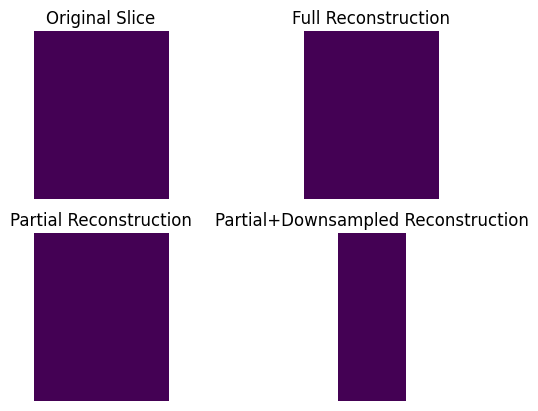
Compare visualizations
We can compare the results of reconstruction. There is no degradation in doing only a partial reconstruction. Downsampling is obviously lower resolution, but the same result as first doing the full reconstruction and then downsampling.
import matplotlib.pyplot as plt

fig, axs = plt.subplots(2, 2, sharey=True)

axs[0, 0].imshow(np.rot90(X[:, 15, :].double().squeeze()), vmin=1, vmax=3)
axs[0, 1].imshow(np.rot90(Xf[:, 15, :].double().squeeze()), vmin=1, vmax=3)
axs[1, 0].imshow(np.rot90(Xslice.double().squeeze()), vmin=1, vmax=3)
axs[1, 1].imshow(np.rot90(Xds.double().squeeze()), vmin=1, vmax=3)

axs[0, 0].set_aspect(aspect="equal")
axs[0, 1].set_aspect(aspect="equal")
axs[1, 0].set_aspect(aspect="equal")
axs[1, 1].set_aspect(aspect="equal")

axs[0, 0].set_axis_off()
axs[0, 1].set_axis_off()
axs[1, 0].set_axis_off()
axs[1, 1].set_axis_off()

axs[0, 0].set_title("Original Slice")
axs[0, 1].set_title("Full Reconstruction")
axs[1, 0].set_title("Partial Reconstruction")
axs[1, 1].set_title("Partial+Downsampled Reconstruction")

axs[1, 1].set_xlim = axs[1, 0].get_xlim()
axs[1, 1].set_ylim = axs[1, 0].get_ylim()